Curve fitting

Fitting of a noisy curve by an asymmetrical peak model, with an iterative process (Gauss–Newton algorithm with variable damping factor α).
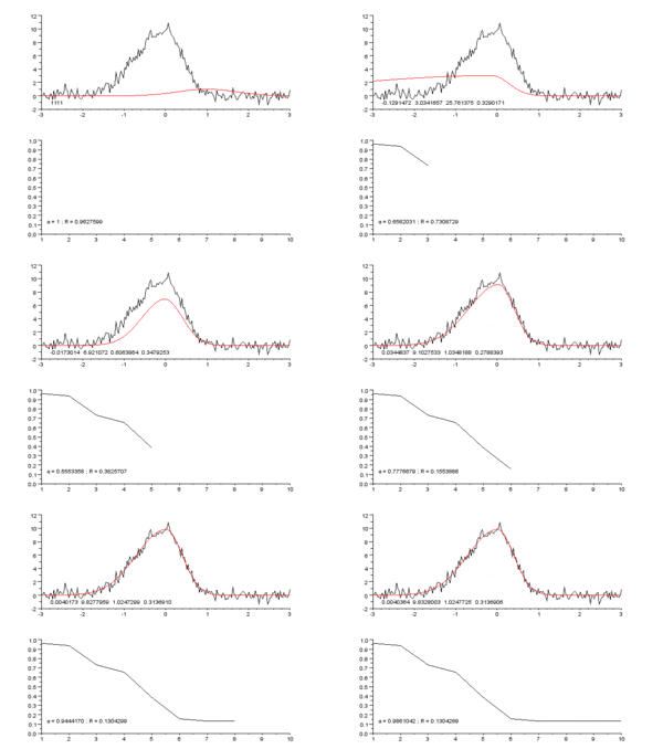
Top: raw data and model.
Bottom: evolution of the normalised sum of the squares of the errors.

Fit approximation
Concepts
Orders of approximation Scale analysis · Big O notation Curve fitting · False precision Significant figures
Other fundamentals
Approximation · Generalization error Taylor polynomial Scientific modelling

Curve fitting^[1][2] is the process of constructing a curve, or mathematical function, that has the best fit to a series of data points,^[3] possibly subject to constraints.^[4][5] Curve fitting can involve either interpolation,^[6][7] where an exact fit to the data is required, or smoothing,^[8][9] in which a "smooth" function is constructed that approximately fits the data. A related topic is regression analysis,^[10][11] which focuses more on questions of statistical inference such as how much uncertainty is present in a curve that is fit to data observed with random errors. Fitted curves can be used as an aid for data visualization,^[12][13] to infer values of a function where no data are available,^[14] and to summarize the relationships among two or more variables.^[15] Extrapolation refers to the use of a fitted curve beyond the range of the observed data,^[16] and is subject to a degree of uncertainty^[17] since it may reflect the method used to construct the curve as much as it reflects the observed data.

Different types of curve fitting

Fitting functions to data points

Most commonly, one fits a function of the form y=f(x).

Fitting lines and polynomial functions to data points

Polynomial curves fitting points generated with a sine function.
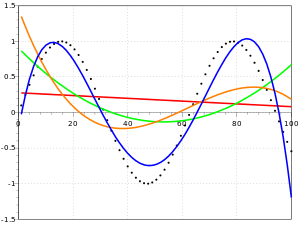
Red line is a first degree polynomial, green line is second degree, orange line is third degree and blue is fourth degree

Starting with a first degree polynomial equation:

This is a line with slope a. A line will connect any two points, so a first degree polynomial equation is an exact fit through any two points with distinct x coordinates.

If the order of the equation is increased to a second degree polynomial, the following results:

This will exactly fit a simple curve to three points.

If the order of the equation is increased to a third degree polynomial, the following is obtained:

This will exactly fit four points.

A more general statement would be to say it will exactly fit four constraints. Each constraint can be a point, angle, or curvature (which is the reciprocal of the radius of an osculating circle). Angle and curvature constraints are most often added to the ends of a curve, and in such cases are called end conditions. Identical end conditions are frequently used to ensure a smooth transition between polynomial curves contained within a single spline. Higher-order constraints, such as "the change in the rate of curvature", could also be added. This, for example, would be useful in highway cloverleaf design to understand the rate of change of the forces applied to a car (see jerk), as it follows the cloverleaf, and to set reasonable speed limits, accordingly.

The first degree polynomial equation could also be an exact fit for a single point and an angle while the third degree polynomial equation could also be an exact fit for two points, an angle constraint, and a curvature constraint. Many other combinations of constraints are possible for these and for higher order polynomial equations.

If there are more than n + 1 constraints (n being the degree of the polynomial), the polynomial curve can still be run through those constraints. An exact fit to all constraints is not certain (but might happen, for example, in the case of a first degree polynomial exactly fitting three collinear points). In general, however, some method is then needed to evaluate each approximation. The least squares method is one way to compare the deviations.

There are several reasons given to get an approximate fit when it is possible to simply increase the degree of the polynomial equation and get an exact match.:

• Even if an exact match exists, it does not necessarily follow that it can be readily discovered. Depending on the algorithm used there may be a divergent case, where the exact fit cannot be calculated, or it might take too much computer time to find the solution. This situation might require an approximate solution.
• The effect of averaging out questionable data points in a sample, rather than distorting the curve to fit them exactly, may be desirable.
• Runge's phenomenon: high order polynomials can be highly oscillatory. If a curve runs through two points A and B, it would be expected that the curve would run somewhat near the midpoint of A and B, as well. This may not happen with high-order polynomial curves; they may even have values that are very large in positive or negative magnitude. With low-order polynomials, the curve is more likely to fall near the midpoint (it's even guaranteed to exactly run through the midpoint on a first degree polynomial).
• Low-order polynomials tend to be smooth and high order polynomial curves tend to be "lumpy". To define this more precisely, the maximum number of inflection points possible in a polynomial curve is n-2, where n is the order of the polynomial equation. An inflection point is a location on the curve where it switches from a positive radius to negative. We can also say this is where it transitions from "holding water" to "shedding water". Note that it is only "possible" that high order polynomials will be lumpy; they could also be smooth, but there is no guarantee of this, unlike with low order polynomial curves. A fifteenth degree polynomial could have, at most, thirteen inflection points, but could also have twelve, eleven, or any number down to zero.

The degree of the polynomial curve being higher than needed for an exact fit is undesirable for all the reasons listed previously for high order polynomials, but also leads to a case where there are an infinite number of solutions. For example, a first degree polynomial (a line) constrained by only a single point, instead of the usual two, would give an infinite number of solutions. This brings up the problem of how to compare and choose just one solution, which can be a problem for software and for humans, as well. For this reason, it is usually best to choose as low a degree as possible for an exact match on all constraints, and perhaps an even lower degree, if an approximate fit is acceptable.

Fitting other functions to data points

Other types of curves, such as trigonometric functions (such as sine and cosine), may also be used, in certain cases.

In spectroscopy, data may be fitted with Gaussian, Lorentzian, Voigt and related functions.

Algebraic fit versus geometric fit for curves

For algebraic analysis of data, "fitting" usually means trying to find the curve that minimizes the vertical (y-axis) displacement of a point from the curve (e.g., ordinary least squares). However for graphical and image applications geometric fitting seeks to provide the best visual fit; which usually means trying to minimize the orthogonal distance to the curve (e.g., total least squares), or to otherwise include both axes of displacement of a point from the curve. Geometric fits are not popular because they usually require non-linear and/or iterative calculations, although they have the advantage of a more aesthetic and geometrically accurate result.^[18][19][20]

Fitting plane curves to data points

If a function of the form cannot be postulated, one can still try to fit a plane curve.

Other types of curves, such as conic sections (circular, elliptical, parabolic, and hyperbolic arcs) or trigonometric functions (such as sine and cosine), may also be used, in certain cases. For example, trajectories of objects under the influence of gravity follow a parabolic path, when air resistance is ignored. Hence, matching trajectory data points to a parabolic curve would make sense. Tides follow sinusoidal patterns, hence tidal data points should be matched to a sine wave, or the sum of two sine waves of different periods, if the effects of the Moon and Sun are both considered.

For a parametric curve, it is effective to fit each of its coordinates as a separate function of arc length; assuming that data points can be ordered, the chord distance may be used.^[21]

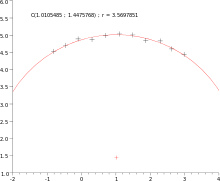
Fitting a circle by geometric fit

Circle fitting with the Coope method, the points describing a circle arc, centre (1 ; 1), radius 4.

different models of ellipse fitting

Ellipse fitting minimising the algebraic distance (Fitzgibbon method).

Coope^[22] approaches the problem of trying to find the best visual fit of circle to a set of 2D data points. The method elegantly transforms the ordinarily non-linear problem into a linear problem that can be solved without using iterative numerical methods, and is hence an order of magnitude faster than previous techniques.

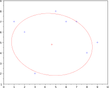
Fitting an ellipse by geometric fit

The above technique is extended to general ellipses^[23] by adding a non-linear step, resulting in a method that is fast, yet finds visually pleasing ellipses of arbitrary orientation and displacement.

Application to surfaces

Note that while this discussion was in terms of 2D curves, much of this logic also extends to 3D surfaces, each patch of which is defined by a net of curves in two parametric directions, typically called u and v. A surface may be composed of one or more surface patches in each direction.

Software

Many statistical packages such as R and numerical software such as the GNU Scientific Library, MLAB, DataMelt Maple, MATLAB, SciPy and OpenOpt include commands for doing curve fitting in a variety of scenarios. There are also programs specifically written to do curve fitting; they can be found in the lists of statistical and numerical analysis programs as well as in Category:Regression and curve fitting software.

See also

• Adjustment of observations
• Curve-fitting compaction
• Estimation theory
• Function approximation
• Goodness of fit
• Levenberg–Marquardt algorithm
• Line fitting
• Nonlinear regression
• Overfitting
• Plane curve
• Probability distribution fitting
• Smoothing
• Splines (interpolating, smoothing)
• Time series
• Total least squares
• Trend estimation

References

Further reading

• N. Chernov (2010), Circular and linear regression: Fitting circles and lines by least squares, Chapman & Hall/CRC, Monographs on Statistics and Applied Probability, Volume 117 (256 pp.).

Wikimedia Commons has media related to Curve fitting.

References

- ↑ Sandra Lach Arlinghaus, PHB Practical Handbook of Curve Fitting. CRC Press, 1994.
- ↑ William M. Kolb. Curve Fitting for Programmable Calculators. Syntec, Incorporated, 1984.
- ↑ S.S. Halli, K.V. Rao. 1992. Advanced Techniques of Population Analysis. ISBN 0306439972 Page 165 (cf. ... functions are fulfilled if we have a good to moderate fit for the observed data.)
- ↑ The Signal and the Noise: Why So Many Predictions Fail-but Some Don't. By Nate Silver
- ↑ Data Preparation for Data Mining: Text. By Dorian Pyle.
- ↑ Numerical Methods in Engineering with MATLAB®. By Jaan Kiusalaas. Page 24.
- ↑ Numerical Methods in Engineering with Python 3. By Jaan Kiusalaas. Page 21.
- ↑ Numerical Methods of Curve Fitting. By P. G. Guest, Philip George Guest. Page 349.
- ↑ See also: Mollifier
- ↑ Fitting Models to Biological Data Using Linear and Nonlinear Regression. By Harvey Motulsky, Arthur Christopoulos.
- ↑ Regression Analysis By Rudolf J. Freund, William J. Wilson, Ping Sa. Page 269.
- ↑ Visual Informatics. Edited by Halimah Badioze Zaman, Peter Robinson, Maria Petrou, Patrick Olivier, Heiko Schröder. Page 689.
- ↑ Numerical Methods for Nonlinear Engineering Models. By John R. Hauser. Page 227.
- ↑ Methods of Experimental Physics: Spectroscopy, Volume 13, Part 1. By Claire Marton. Page 150.
- ↑ Encyclopedia of Research Design, Volume 1. Edited by Neil J. Salkind. Page 266.
- ↑ Community Analysis and Planning Techniques. By Richard E. Klosterman. Page 1.
- ↑ An Introduction to Risk and Uncertainty in the Evaluation of Environmental Investments. DIANE Publishing. Pg 69
- ↑ Ahn, Sung-Joon (December 2008), "Geometric Fitting of Parametric Curves and Surfaces" (PDF), Journal of Information Processing Systems, 4 (4), doi:10.3745/JIPS.2008.4.4.153
- ↑ Chernov, N.; Ma, H. (2011), "Least squares fitting of quadratic curves and surfaces", in Yoshida, Sota R., Computer Vision, Nova Science Publishers, pp. 285–302, ISBN 9781612093994
- ↑ Liu, Yang; Wang, Wenping (2008), "A Revisit to Least Squares Orthogonal Distance Fitting of Parametric Curves and Surfaces", in Chen, F.; Juttler, B., Advances in Geometric Modeling and Processing, Lecture Notes in Computer Science, 4975, pp. 384–397, doi:10.1007/978-3-540-79246-8_29, ISBN 978-3-540-79245-1
- ↑ p.51 in Ahlberg & Nilson (1967) The theory of splines and their applications, Academic Press, 1967
- ↑ Coope, I.D. (1993). "Circle fitting by linear and nonlinear least squares". Journal of Optimization Theory and Applications. 76 (2): 381. doi:10.1007/BF00939613.
- ↑ Paul Sheer, A software assistant for manual stereo photometrology, M.Sc. thesis, 1997